Multidimensional quadrature bases

In some cases, simple one-dimensional discrete variable representation bases (see Discrete-variable representation (DVR) bases), or direct products thereof, cannot suitably represent a wavefunction. This is usually due to the need to satisfy certain boundary conditions, as we will see with examples below. NITROGEN implements a variety of other types of basis functions with the NDBasis class to meet this need. Each basis set comes with a suitable grid of quadrature points and weights to calculate matrix element integrals involving the basis functions. The basis functions themselves are implemented as differentiable DFun objects, so that integrals involving the derivatives of the basis functions can also be evaluated.

Let’s explore some features of NDBasis objects with a basis set built with the radial eigenfunctions of a d-dimensional isotropic harmonic oscillator.

>>> import nitrogen as n2
>>> basis = n2.basis.RadialHOBasis(5, 2.5, 0)
>>> basis.nd # The number of dimensions
1
>>> basis.Nb # The number of basis functions
6

The basis functions can be explicitly evaluated with the basisfun attribute, which is a DFun object.

>>> basis.basisfun.nx == basis.nd
True
>>> basis.basisfun.nf == basis.Nb
True

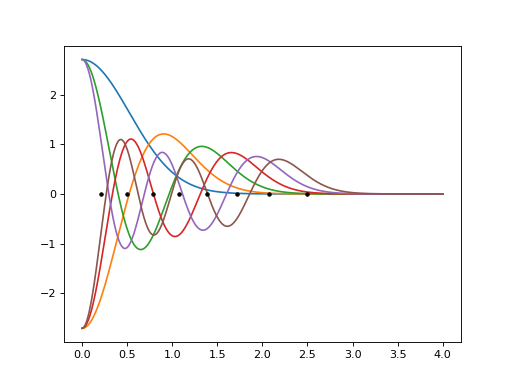
This example plots the basis set functions and the quadrature grid points:

import nitrogen as n2
import matplotlib.pyplot as plt
import numpy as np

basis = n2.basis.RadialHOBasis(5, 2.5, 0)
r = np.linspace(0, 4, 500) # make a grid for plotting
y = basis.basisfun.val(r.reshape((1,-1))) # evaluate basis
plt.plot(r, y.T,'-') # plot the basis functions
plt.plot(basis.qgrid[0],0*basis.qgrid[0],'k.') # plot the quad. grid

(Source code, png, hires.png, pdf)

Matrix elements of the basis functions are defined with respect to a volume element weight function, \(\Omega\)

\[\langle \phi_i \vert \phi_j \rangle = \int d\vec{x}\,\Omega(\vec{x}) \phi_i(\vec{x}) \phi_j(\vec{x}),\]

The weight function, if needed, can be evaluated with the wgtfun attribute, another DFun object. Integrals can be approximated with a weighted sum over \(N_q\) quadrature grid points \(\vec{x}_k\),

\[\int d\vec{x}\, \Omega(\vec{x}) f(\vec{x}) \approx \sum_{k=0}^{N_q-1} w_k f(\vec{x}_k),\]

where \(w_k\) are the quadrature weights, stored in the wgt attribute.

When an NDBasis object is created, the basis functions are automatically evaluated over the quadrature grid and stored in the bas attribute.

>>> basis_on_grid = basis.basisfun.val(basis.qgrid)
>>> np.allclose(basis_on_grid, basis.bas)
True

The quadrature rule can be used to evaluate the overlap integrals of the basis functions verify that the basis is orthonormal.

>>> phi = basis.bas # The basis functions on the quad. grid
>>> w = basis.wgt # The quad. weights
>>> S = (phi * w) @ phi.T # The overlap integrals
>>> np.allclose(S, np.eye(basis.Nb)) # S equals identity?
True

Most NDBasis sub-classes have optional keywords to control the number of quadrature points. Generally, the default values are appropriate for most cases, but these can be changed if necessary.

Let’s move on to a two-dimensional example, the real spherical harmonics, which are defined by the RealSphericalH special function class.

>>> basis = n2.basis.RealSphericalHBasis(2,2)  # (max m, max l)
>>> basis.nd  # (theta, phi) coordinates
2
>>> basis.m # The "real" m quantum number
array([-2, -1, -1,  0,  0,  0,  1,  1,  2])
>>> basis.l # The l quantum number
array([2, 1, 2, 0, 1, 2, 1, 2, 2])

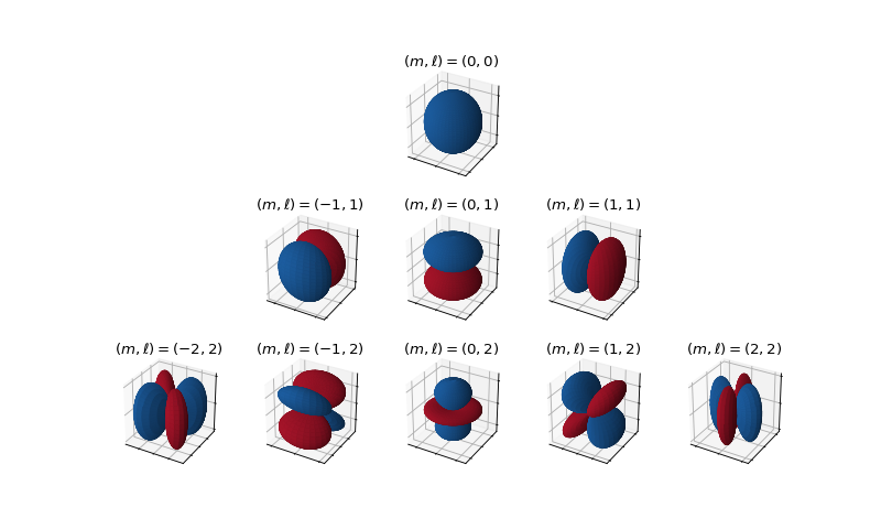
These basis functions plotted in spherical coordinates look like

(Source code, png, hires.png, pdf)

As with the previous example, we can verify that the basis is orthonormal

>>> Y = basis.bas # the real sph. harmonic basis functions on the quad. grid
>>> w = basis.wgt # the quadrature weights
>>> S = (Y * w) @ Y.T # the overlap matrix
>>> np.allclose(S, np.eye(basis.Nb))
True

The real spherical harmonics are eigenfunctions of the total angular momentum operator, i.e.

\[-\frac{\partial^2}{\partial \theta^2} - \cot \theta \frac{\partial}{\partial \theta} - \frac{\partial_\phi^2}{\sin^2\theta}\]

with eigenvalue \(\ell(\ell+1)\). We can verify this numerically by evaluating the matrix elements of this differential operator using the quadrature weights.

# Evaluate the derivatives of the basis functions up to second order
>>> dY = basis.basisfun.f(basis.qgrid, deriv = 2)
>>> dY_th = dY[1] # theta derivative
>>> dY_thth = 2 * dY[3] # theta/theta derivative
>>> dY_phph = 2 * dY[5] # phi/phi derivative
>>> cot = 1/np.tan(basis.qgrid[0]) # cot(theta) on quad. grid
>>> sin2 = np.sin(basis.qgrid[0])**2 # sin**2(theta) on quad. grid
>>> DY = -dY_thth - cot * dY_th - dY_phph/sin2 # The diff. op
>>> D = (Y * w) @ DY.T # matrix elements of diff. op
>>> l = basis.l # The l quantum number of each basis function
>>> np.allclose(D, np.diag(l*(l+1)))
True