Discrete-variable representation (DVR) bases

A discrete-variable representation (DVR) is a grid-based, coordinate-localized basis set. A variety of DVRs are used for problems in nuclear motion theory (and many other areas of chemical and molecular physics). Their primary benefit is that coordinate operators are approximately diagonal in the DVR, simplifying matrix element integrals considerably. This tutorial will not discuss the mathematical details of DVR bases. A valuable review by Light and Carrington is available here.

DVR bases in NITROGEN are implemented with the GenericDVR class in the nitrogen.basis module. Commonly used DVR bases can be generated with the SimpleDVR constructor by specifying just the grid range, size, and DVR type.

>>> import nitrogen as n2
>>> my_dvr = n2.basis.SimpleDVR(start=-1.0, stop=1.0, num=11, basis='ho')
>>> my_dvr.grid # the DVR grid points
array([-1.00000000e+00, -7.58705798e-01, -5.52259538e-01, -3.61610366e-01,
       -1.79041785e-01,  6.81988078e-17,  1.79041785e-01,  3.61610366e-01,
        5.52259538e-01,  7.58705798e-01,  1.00000000e+00])

We do not usually need to evaluate the actual DVR basis functions themselves. Nonetheless, GenericDVR objects provide a wfs() method (i.e. “wavefunctions”) to calculate them. This is especially useful for plotting.

import nitrogen as n2
import matplotlib.pyplot as plt
import numpy as np

my_dvr = n2.basis.SimpleDVR(start=-1.0, stop=1.0, num=11, basis='ho')
x = np.linspace(-3,3,251) # make a grid for plotting
y = my_dvr.wfs(x)
plt.plot(x,y[:,[0,-1]],'-')
plt.plot(my_dvr.grid, np.zeros_like(my_dvr.grid), 'k.')

(Source code, png, hires.png, pdf)

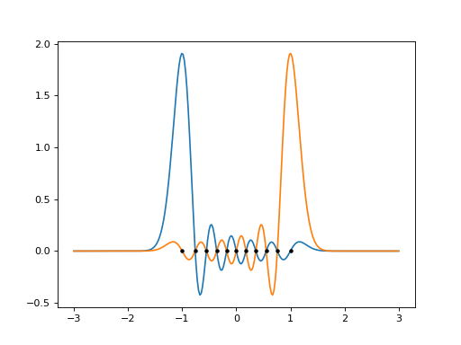
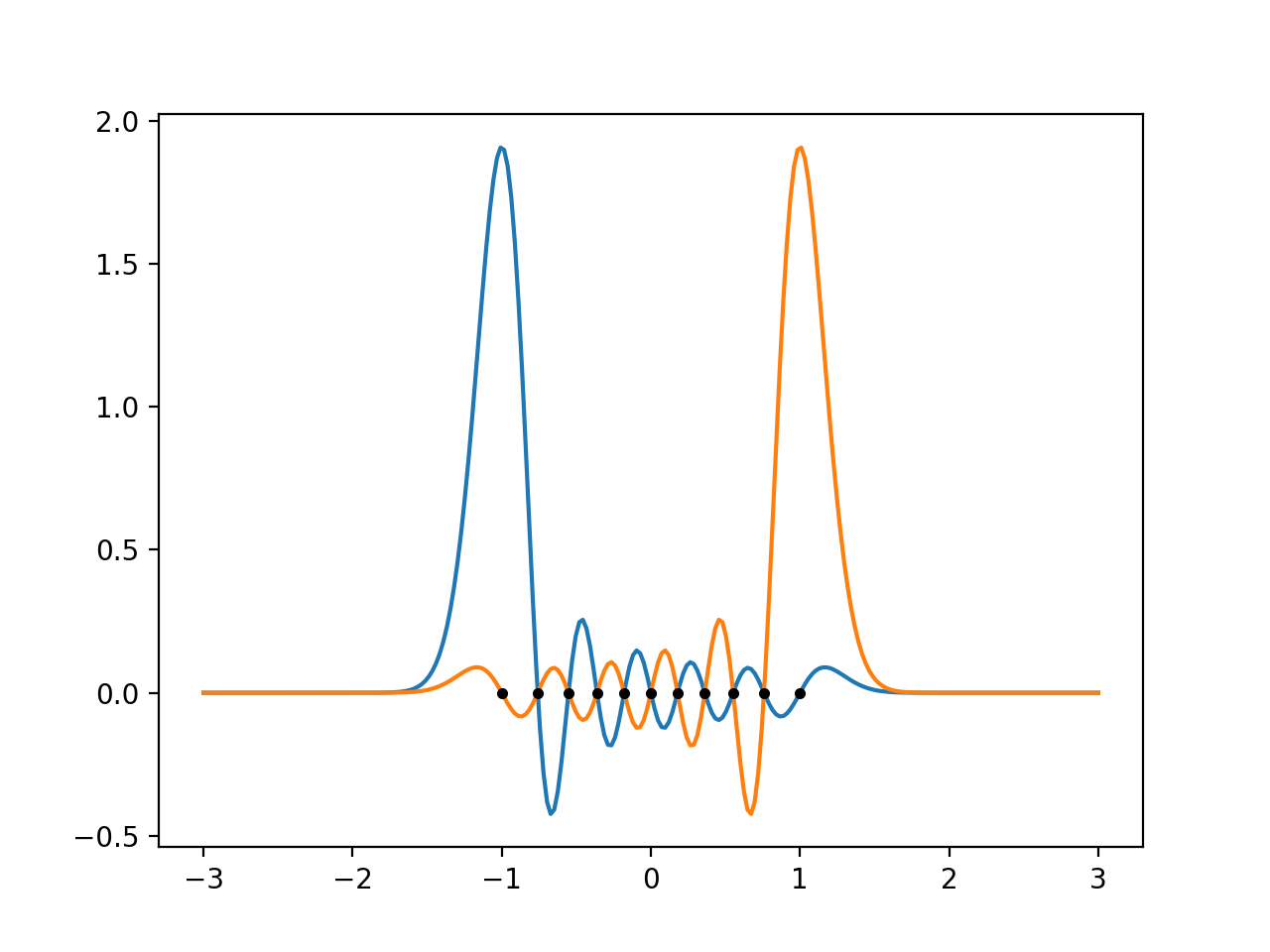
This plot illustrates the local \(\delta\)-like character of DVR functions and the general feature that they possess nodes at the DVR grid points.

A GenericDVR object also provides the DVR representations of the first and second derivative operators.

>>> my_dvr.D[:4,:4] # a bit of the first derivative operator
array([[ 0.        ,  4.14431839, -2.23343675,  1.56644147],
       [-4.14431839,  0.        ,  4.84387561, -2.51828634],
       [ 2.23343675, -4.84387561,  0.        ,  5.24523651],
       [-1.56644147,  2.51828634, -5.24523651,  0.        ]])
>>> my_dvr.D2[:4,:4] # a bit of the second derivative operator
array([[-36.07699265,  27.62191064,  -3.24764022,  -1.82136139],
       [ 27.62191064, -61.69581227,  40.19742261,  -5.95469296],
       [ -3.24764022,  40.19742261, -78.0345033 ,  48.29617288],
       [ -1.82136139,  -5.95469296,  48.29617288, -88.55262844]])

These quantities make it simple to set up coordinate-representation Hamiltonians. For example, consider the 1D harmonic oscillator with \(\hbar = \omega = m = 1\),

\[ \begin{align}\begin{aligned}H &= T + V(x)\\&= -\frac{1}{2} \frac{d^2}{dx^2} + \frac{1}{2} x^2.\end{aligned}\end{align} \]

This example sets up the corresponding DVR Hamiltonian using a sinc-DVR basis:

>>> dvr = n2.basis.SimpleDVR(-7, 7, 35, basis = 'sinc')
>>> V = np.diag(0.5 * (dvr.grid)**2) # potential energy matrix
>>> T = -0.5 * dvr.D2 # kinetic energy matrix
>>> H = T + V
>>> w,u = np.linalg.eigh(H) # calculate spectrum
>>> w[:5] # the first five eigenenergies (1/2, 3/2, 5/2, ...)
array([0.5, 1.5, 2.5, 3.5, 4.5])

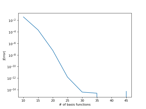
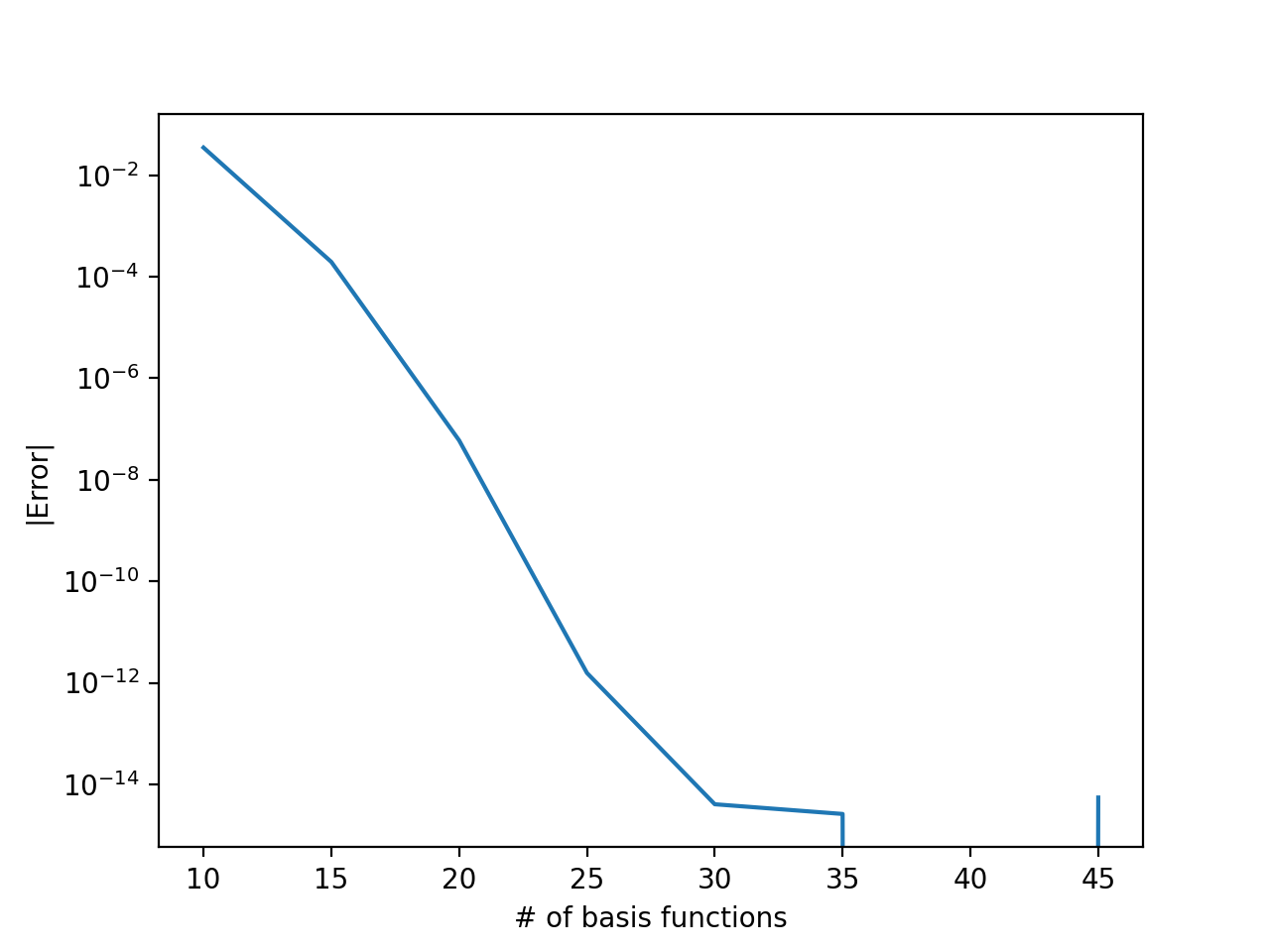
The convergence with respect to the number of DVR basis functions (i.e. the density of the grid points) is usually exponential.

import nitrogen as n2
import numpy as np
import matplotlib.pyplot as plt

err = []
for N in range(10, 50, 5):
    dvr = n2.basis.SimpleDVR(-7, 7, N, basis = 'sinc')
    V = np.diag(0.5 * (dvr.grid)**2)
    T = -0.5 * dvr.D2
    H = T + V
    w,_ = np.linalg.eigh(H)
    err.append(w[0] - 0.5) # record error relative to exact energy
err = np.array(err)
plt.plot(range(10,50,5), np.abs(err))
plt.yscale('log')
plt.xlabel('# of basis functions')
plt.ylabel('|Error|')

(Source code, png, hires.png, pdf)

Full matrix representations of higher-dimensional direct-product DVR grids can be constructed with numpy.kron(). This is practical for low dimensions, but does not take advantage of the sparse nature of DVR operators, for which a LinearOperator may be more appropriate.

The nitrogen.basis.SimpleDVR constructor provides for several common primitive DVR types (basis = 'sinc', 'ho', 'fourier', 'lengendre', …), an important difference between which is the boundary conditions they satisfy. For example, the fourier DVR is periodic over the grid range. The derivative operator of a legendre DVR is not strictly anti-Hermitian because of non-zero boundary terms (and, in fact, its D2 attribute equals the \(-\partial^\dagger \partial\) operator, which is not equivalent to \(\partial^2\) in this case). Care should always be taken to consider the detailed boundary conditions, but for most problems with no special issues (i.e. \(\psi \rightarrow 0\) in a “suitable” way) sinc and ho DVRs are appropriate.